Getting Started

Download and Installation

This guide assumes that you have access to an administrator or sudoer account on a macOS or Linux system.

Getting Organized

Creating Enclosing Directory

Create a vivarium_work folder anywhere you like. But for installing some third-party software, everything we do will occur inside this folder.

Setting PYTHONPATH

Vivarium needs the root of the repository to be in your PYTHONPATH environment variable so that Python can find Vivarium. To make this easy to set, we suggest adding this line to your shell startup file:

alias pycd='export PYTHONPATH="$PWD:$PYTHONPATH"'

Now when you are about to work on Vivarium, navigate to the root of the Vivarium repository (vivarium_work/vivarium) and run pycd in your terminal. You will need to do this for each terminal window you use.

Installing Dependencies

Below, we list the dependencies Vivarium requires, how to check whether you have them, how to install them, and in some cases, how to set them up for Vivarium. Make sure you have each of them installed.

Python 3

We wrote Vivarium in Python 3. While we did also write it to be Python-2-compatible, the Python Software Foundation has deprecated Python 2, so we strongly recommend using Python 3.

Check Installation

$ python --version
Python <version>

Make sure you see a version at least 3.6.

Install

Download the latest installer from the Python download page

Open JDK 8

Zookeeper and Kafka, which we will address later, require that you have Java installed.

Check Installation

$ java -version
java version <version> <date>

Ensure the version is at least 1.8.

Install

Download the latest JDK installer from the Java SE Downloads site. As of writing the latest is Java SE 14. Download and run the appropriate installer for your platform. Then you need to set the JAVA_HOME environment variable, for instance by adding export JAVA_HOME=$(/usr/libexec/java_home) to your startup shell file (e.g. ~/.bash_profile or ~/.profile).

Zookeeper and Kafka

Kafka is a message passing system that allows decoupling of message senders and message receivers. It does this by providing two abstractions, a Consumer and a Producer. A Consumer can subscribe to any number of “topics” it will receive messages on, and a Producer can send to any topics it wishes. Topics are communication “channels” between processes that otherwise do not need to know who is sending and receiving these messages. Vivarium uses Kafka to pass messages between actors, for example between a cell and its environment.

Kafka relies on Zookeeper, which synchronizes access to a hierarchy of key-value pairs called nodes. We like Kafka because it will let us distribute the model across computers in a server cluster, but you can also run a local Kafka instance for development.

Check Installation

For this guide, we will not install Kafka globally on your system. Instead, we will store the Kafka program in vivarium_work and run the executable directly. This means you almost certainly need to install it, even if you use Kafka already.

Install

1. Download Kafka from the Apache Kafka site, choosing the latest version. This will give you a .tgz archive file that includes both Kafka and Zookeeper.

2. Unarchive this file into vivarium_work to create a folder like vivarium_work/kafka_2.11-2.0.0/. Your folder name will likely change slightly to match your version of Kafka.

3. Create a shell script vivarium_work/zookeeper.sh with the following content:

   #!/bin/bash
   
   ./kafka_2.11-2.0.0/bin/zookeeper-server-start.sh \
       ./kafka_2.11-2.0.0/config/zookeeper.properties
   

4. Create a shell script vivarium_work/kafka.sh with the following content:

   #!/bin/bash
   
   ./kafka_2.11-2.0.0/bin/kafka-server-start.sh \
       ./kafka_2.11-2.0.0/config/server.properties \
       --override listeners=PLAINTEXT://127.0.0.1:9092
   

   Overriding the “listeners” address like this allows connections to the Kafka server to withstand network DHCP address changes and the like.

5. Make the scripts executable like this:

   $ chmod 700 vivarium_work/kafka.sh
   $ chmod 700 vivarium_work/zookeeper.sh
   

   Now you can start and stop the Zookeeper and Kafka servers like this:

   $ vivarium_work/zookeeper.sh
   $ vivarium_work/kafka.sh
   

   Make sure to start Zookeeper before Kafka, as Kafka expects a Zookeeper instance to already be running when in starts. Also note that you must run these two commands in separate terminals. To shut them down, you can just use CTRL-C to kill the processes.

   Warning

   Make sure you shut down Kafka before Zookeeper! If you shut down Zookeeper first, Kafka will refuse to quit. You can then force it to stop with kill -9.

MongoDB

We use a MongoDB database to store the data collected from running simulations. This can be a remote server, but for this guide we will run a MongoDB server locally.

Check Installation

$ mongod --version
db version v4.2.3
...

Make sure you see a version at least 4.2.

Install

If you are on macOS, you can install MongoDB using Homebrew. You will need to add the MongoDB tap following the instructions here.

If you are on Linux, see the MongoDB documentation’s instructions.

Setup

You can get a MongoDB server up and running locally any number of ways. Here is one:

1. Create a folder vivarium_work/mongodb. This is where MongoDB will store the database We store the database here instead of at the default location in /usr/local/var/mongodb to avoid permissions issues if you are not running as an administrator.

2. Make a copy of the mongod configuration file so we can make changes:

   $ cp /usr/local/etc/mongod.conf vivarium_work/mongod.conf
   

   Note that your configuration file may be somewhere slightly different. Check the MongoDB documentation for your system.

3. In vivarium_work/mongod.conf change the path after dbPath: to point to vivarium_work/mongodb.

4. Create a shell script vivarium_work/mongo.sh with the following content:

   #!/bin/bash
   
   mongod --config mongodb.conf
   

5. Make the script executable:

   $ chmod 700 vivarium_work/mongo.sh
   

   Now you can launch MongoDB by running this script:

   $ vivarium_work/mongo.sh
   

GNU Linear Programming Kit (GLPK)

One of the Python packages we will install later, swiglpk, requires that you already have GLPK installed on your system.

Check Installation

We don’t have a way to check whether you have glpk installed. If you think you already have it, you can proceed with the installation and watch for an error about missing glpk.

Install

If you use Homebrew, you can install GLPK like this:

$ brew install glpk

Otherwise, follow the installation instructions on the GLPK homepage.

Leiningen

Our simulation runs each cell on its own thread, and we use Leiningen to manage these threads.

Check Installation

To check whether you have Leiningen installed, run:

$ lein --version
Leiningen <version> ...

You may also see a deprecation warning from Java HotSpot, which you can ignore. Make sure the version is at least 2.9.

Install

To install Leiningen, follow the instructions on its website. You can also install the leiningen formula on Homebrew instead.

Download and Setup Vivarium

Download the Code

The Vivarium code is available on GitHub. Move into your vivarium_work directory and clone the repository to download the code

$ cd vivarium_work
$ git clone https://github.com/CovertLab/vivarium.git

This will create a vivarium folder inside vivarium_work. All the code for Vivarium is inside this vivarium folder.

Installing Python Packages

Above we installed all the non-Python dependencies, but we still have to install the Python packages Vivarium uses.

1. Move into the vivarium folder created when you cloned the repository.

2. (optional) Create and activate a virtual environment:

   $ python3 -m venv venv
   ...
   $ source venv/bin/activate
   

3. Install Numpy. One of our dependencies, stochastic-arrow requires that Numpy be installed first. Check the requirements.txt file for a line like this:

   numpy==1.15.3
   

   Now install the version of Numpy specified in requirements.txt

   $ pip install numpy==1.15.3
   

4. Install packages

   $ pip install -r requirements.txt
   

   If you encounter problems installing numpy and/or scipy, try this instead:

   $ pip install -r requirements.txt --no-binary numpy,scipy
   $ pip install numpy
   $ pip install scipy
   

Now you are all set to run Vivarium!

Run Simulations

Some Terminology: Processes and Composites

In Vivarium, we break our cell models into processes. Each process models part of the cell’s function. For example, we have processes for metabolism, transcription, and translation in Vivarium. We can combine these processes into compartments that model a cell with all the functionality modeled by the included processes. For example, we could compose transcription and translation to create a fuller gene expression model.

In Vivarium, we store individual processes in vivarium/vivarium/processes and compartments of processes in vivarium/vivarium/compartments.

Running Processes and Composites in Isolation

You can run any process or compartment by itself. While this is too simple for modeling whole cells or colonies, simulating processes in isolation lets you study their dynamics and tune them to different conditions. To run a process or compartment, you can execute the Python file that defines it. For example, we can run the degradation process like this:

$ python vivarium_work/vivarium/vivarium/processes/degradation.py
...

Tip

If you get errors from Python about being unable to find vivarium, make sure you’ve added the repository root to your PYTHONPATH. See Setting PYTHONPATH for details.

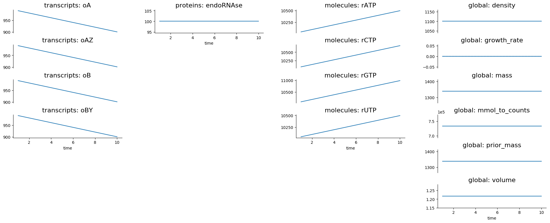
Don’t worry about the output–it’s for developers. You will see a new folder at vivarium_work/vivarium/vivarium/out/tests. This is where we store the output from running processes and compartments in isolation. For the degradation process, the output is in the degradation folder inside tests. Here you’ll find a simulation.png file that looks like this:

If you wanted to understand how the degradation process works, this would show you that it removes transcripts and returns the RNA nucleotides to the cell.

Some processes also produce the data shown in the plots. You can find this data in simulation_data.csv. Try running the convenience_kinetics process to see how this works!

Lastly, try running the flagella_expression compartment like this:

$ python vivarium_work/vivarium/vivarium/compartments/flagella_expression.py

Now in the flagella_expression_composite (the suffix _composite is left over from when we called compartments “composites”) in tests, you should see an image containing a plot like this:

Notice that even from this minimal simulation, we can tell which amino acid is limiting! In this case the colors are so similar that it’s hard to tell, but the limiting amino acid is either alanine or leucine.

Running Agents in Terminal Windows

Tip

Running agents separately in terminal windows is helpful for debugging because it lets you see the output from each agent.

Terminology: Agents

Vivarium is heavily influenced by agent-based modeling, in which the model consists of individual agents interacting with each other. In Vivarium, cells are agents that move around and grow within a shared environment. These agents interact with each other and their environment by passing messages through Kafka.

How to Run Agents

Each agent runs on its own thread. We do this because each agent can be as complex as an entire whole-cell model, so the entire simulation cannot run on a single thread. Shepherd can manage these threads for you; importantly, you must use Shepherd if your simulation will require creating or deleting threads. Cell division, for example, involves stopping the mother cell’s thread and starting two new threads, one for each daughter cell, so division requires Shepherd.

That said, you can run agents on your own instead of using Shepherd.

Warning

If you run a simulation using this method that includes stopping and/or starting agents, the agents will stop, but new ones will not start. For example if your cell divides, the agent you started for the mother cell will stop, but the daughter cells will not start.

We will run each agent in its own terminal window to mimic the threads that Shepherd would create. Let’s see how!

First we need to get all our servers running. Do each of the following in a separate terminal window:

1. Start Zookeeper:

   $ vivarium_work/zookeeper.sh
   ...
   ... INFO binding to port 0.0.0.0/0.0.0.0:2181 ...
   

2. Start Kafka:

   $ vivarium_work/kafka.sh
   ...
   ... INFO [KafkaServer id=0] started (kafka.server.KafkaServer)
   

   You should also see som text print out on the Zookeeper window. You might see some NoNode warnings–these are safe to ignore.

   Warning

   You must start Zookeeper before Kafka!

3. Start MongoDB:

   $ vivarium_work/mongo.sh
   

   There shouldn’t be any output.

   If you installed MongoDB using Homebrew, you can instead tell Homebrew to always run a MongoDB server by running:

   $ brew services start mongodb/brew/mongodb-community
   

   Now a MongoDB server will start automatically once you login. Then you can skip the step of starting MongoDB in the future.

Now we can create our agents. We create an agent like this:

$ python -m vivarium.environment.boot --type <type> --id <id> [--outer-id <outId>]

Tip

If you get errors from Python about being unable to find vivarium, make sure you’ve added the repository root to your PYTHONPATH. See Setting PYTHONPATH for details.

where <type> is the agent type, <id> is the identifier for this agent, and <outId> is an optional argument that instructs Vivarium to place the new agent inside the agent with identifier <outId>. This outer agent will almost always be an environment. You can also provide an optional --config '{...}' argument you can use to configure the agent.

To see the other agent types, check out the help text like this:

$ python -m vivarium.environment.boot --help

Here’s an example of running a simulation of a simple environment with three cells that consume glucose and lactose. We will initialize the environment with glucose and lactose, and as the cells deplete the glucose we should see the cells shift to consuming lactose.

1. First, let’s create a ecoli_core_glc environment agent. This is a kind of lattice environment. Lattice environments discretize the simulation space into a two-dimensional grid, each region of which has the same depth. Each region has uniform metabolite concentrations, but metabolite concentrations differ between regions, letting us model a continuous distribution of concentrations. A diffusion process in the environment tends to make the space homogeneous. We start this agent like this:

   $ python -m vivarium.environment.boot --type ecoli_core_glc --id env
   environment started
   

   Warning

   Wait for the environment started to show up before proceeding. Otherwise there won’t be an environment to add the cells to!

2. Next, let’s create three cell agents. These agents will be of type shifter because they will initially consume glucose, but when glucose concentrations drop, they will start consuming lactose. We create these agents like this:

   $ python -m vivarium.environment.boot --type shifter --id c1 --outer-id env
   $ python -m vivarium.environment.boot --type shifter --id c2 --outer-id env
   $ python -m vivarium.environment.boot --type shifter --id c3 --outer-id env
   

   After creating each cell agent, you should see in both the cell and the environment’s terminal windows a message from the cell to the environment declaring itself:

   <-- environment-receive CELL_DECLARE [shifter c1]: {'event':
   'CELL_DECLARE', 'agent_id': 'env', 'inner_id': 'c1',
   'agent_config': { ... }, 'state': {'volume': 1.0}}
   

   And a message from the environment back to the cell:

   <-- cell-receive ENVIRONMENT_SYNCHRONIZE [glc_lct env]:
   {'event': 'ENVIRONMENT_SYNCHRONIZE', 'inner_id': 'c1',
   'outer_id': 'env', 'state': { ... }}
   

3. Now we can start the simulation!

   $ python -m vivarium.environment.control run --id env
   

   Simulations stop on their own once the environment agent hits the end of its programmed timeline. You can also pause, run, and shutdown the simulation like this:

   $ python -m vivarium.environment.control pause --id env
   $ python -m vivarium.environment.control run --id env
   $ python -m vivarium.environment.control shutdown
   

   In this example, one of the cells tries to divide, halting the simulation. We’ll see later how to simulate division.

4. Once the simulation completes, run the analysis script to plot the data:

   $ python vivarium/analysis/run_analysis -e env
   

   When the script completes, look for a folder named env in vivarium_work/vivarium/out with plots from your simulation.

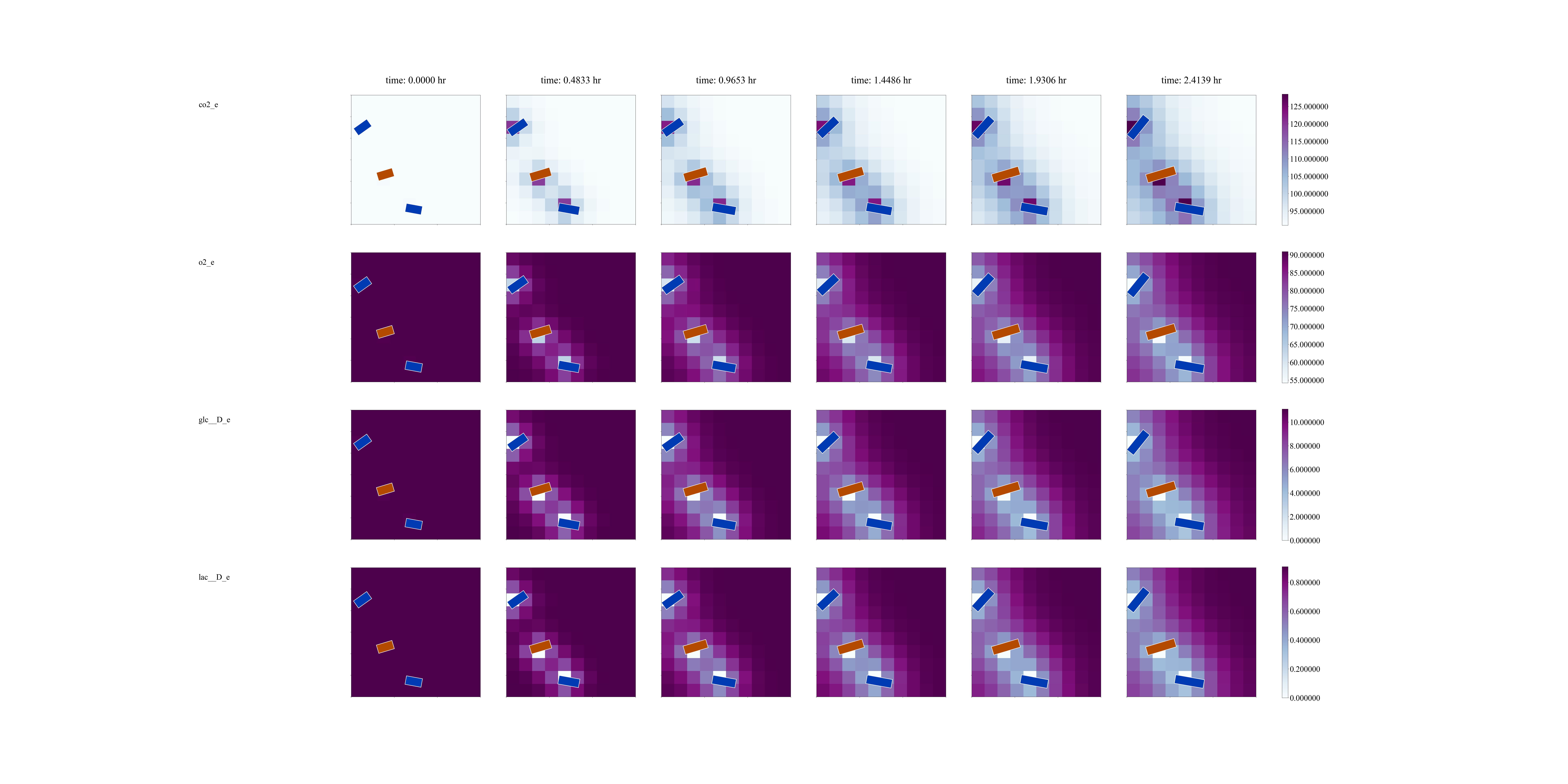
In snap_out.png you should see something like this:

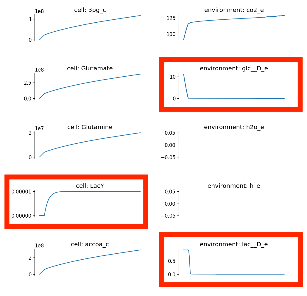
Notice that the cells are consuming glucose and lactose as we expected! Now take a look at c1/compartment.png. Here is part of the plot you should see:

Here notice that the glucose levels near the cells drop precipitously, after which LacY expression increases. Then, the cell consumes the surrounding glucose, as we expected.

Using Shepherd

The usual way to start the simulation is to use Shepherd, which spawns agents in new threads as requested via Kafka messages so you don’t have to launch each agent in its own terminal tab. Furthermore, this enables cell division wherein a cell agent process ends and two new ones begin. To debug an agent, though, see the Running Agents in Terminal Windows instructions above.

Let’s take a look at an example of using Shepherd. We’ll be able to model cells dividing!

1. First, start Zookeeper, Kafka, and MongoDB as we discussed above in How to Run Agents.

2. Launch Shepherd in a separate terminal window:

   $ lein run
   

3. For our environment, let’s make a lattice agent:

   $ python -m vivarium.environment.boot --type ecoli_core_glc --id env2
   environment started
   

   Warning

   Wait for the environment started to show up before proceeding. Otherwise there won’t be an environment to add the cells to!

   Tip

   If you get errors from Python about being unable to find vivarium, make sure you’ve added the repository root to your PYTHONPATH. See Setting PYTHONPATH for details.

4. Next, let’s create a cell agent of type growth_division, which can grow and divide.

   $ python -m vivarium.environment.boot --type growth_division --id c --outer-id env2
   

5. Now we can start the simulation!

   $ python -m vivarium.environment.control run --id env2
   

   This simulation is quite long, so feel free to cancel it with CTRL-C after you’re tired of waiting.

6. Once the simulation finishes, we can analyze the data:

   $ python vivarium/analysis/run_analysis -e env2
   

   Note

   You can run the analysis script while the simulation is still running too.

First, notice the folders in the analysis output. Each folder is a cell, so since the cells divided, we have a lot of them! If you take a look at snap_out.png, you should see rows of plots like this:

Running Experiments

With Shepherd, you can also run experiments that pre-define the environment and cell types. For example, let’s see how we could have run a simulation of growing and dividing cells like above with less work:

1. First, start Zookeeper, Kafka, and MongoDB as we discussed above in How to Run Agents.

2. Now start up Shepherd:

   $ lein run
   

3. Load the experiment:

   Danger

   This experiment doesn’t work yet. We are working on a fix in #178

   $ python -m vivarium.environment.control \
       growth-division-experiment --experiment_id exp
   

   Tip

   If you get errors from Python about being unable to find vivarium, make sure you’ve set your PYTHONPATH to include vivarium. See Setting PYTHONPATH for details.

4. Run the simulation:

   $ python -m vivarium.environment.control run --id exp
   

5. When it finishes, run the analysis:

   $ python vivarium/analysis/run_analysis -e exp
   

   This is a long experiment, so you might want to end the simulation before it finishes.

In snap_out.png, we see a similar outcome to before. The plots are different this time because there is some stochasticity in the model.