Environmental Compartments
In the processes and compartments we have discussed so far, we have assumed that the locations of molecules tracked in stores were unimportant. This assumption breaks down for some parent compartments like environments whose modeled space is too large to be homogenized by diffusion faster than the model’s timestep. To model this spatial heterogeneity, we employ space discretization, diffusion processes, and multi-body physics.
Environments as Compartments
We model environments as compartments with an agents store
and a fields store. The diffusion and multibody physics processes we
discuss below operate on these stores, and the compartments for the
cells in the environment plug their boundary stores into
agents and read from fields.
Space Discretization with Lattice
We model heterogeneous distributions of molecules throughout space by discretizing space into a grid. For each rectangle in the grid, we track the concentrations of all the molecules in the compartment. We also track which rectangle each child compartment is in.
Note
A child compartment is always modeled as being in exactly one rectangle in the grid even if the cell extends into other rectangles. The cell’s position is defined as the position of its midpoint.
Note
You may see child compartments referred to as “agents” because each parent compartment can be thought of as running an agent-based model.
Boundary Stores in Lattice
We tell each cell about the concentrations of molecules using variables in the boundary store. When a cell imports or exports a molecule, it stores the flux in the boundary store. The molecules are then removed from or added to the rectangle in which the cell resides. The flux between cells and their environment is called exchange.
Note
We localize the impact of exchange on the environment to just the cell’s immediate vicinity to allow cells to locally deplete resources or let extruded toxins accumulate.
Diffusion
Of course, just because a cell deposits extruded molecules around itself doesn’t mean those molecules stay localized! We created processes to model diffusion. We have two kinds of diffusion processes:
Diffusion Field
A diffusion field operates on a grid like that described above with
lattice. The diffusion rate is
configurable. See vivarium.processes.diffusion_field for
details.
Diffusion Network
A diffusion network models diffusion between membrane-separated regions. The diffusion network operates on a graph whose nodes are the regions, which are internally homogeneous, and whose edges are the membranes through which molecules can diffuse. You can configure how quickly each molecule can diffuse through each membrane.
In theory, a diffusion field could be modeled as a diffusion network; however, diffusion networks are more computationally intensive to model. Instead, diffusion networks can be used to model diffusion between a cell and its environment through the membrane or a channel.
See vivarium.processes.diffusion_network for details.
Multi-Body Physics
When cells share the same physical space, they will exclude each other. Thermal energy from the environment also buffets the cells. We use a multi-body physics engine to model these forces between compartments. This process applies forces when two compartments overlap by too much and small random forces to approximate thermal jitter.
This process is implemented in
vivarium.processes.multibody_physics.
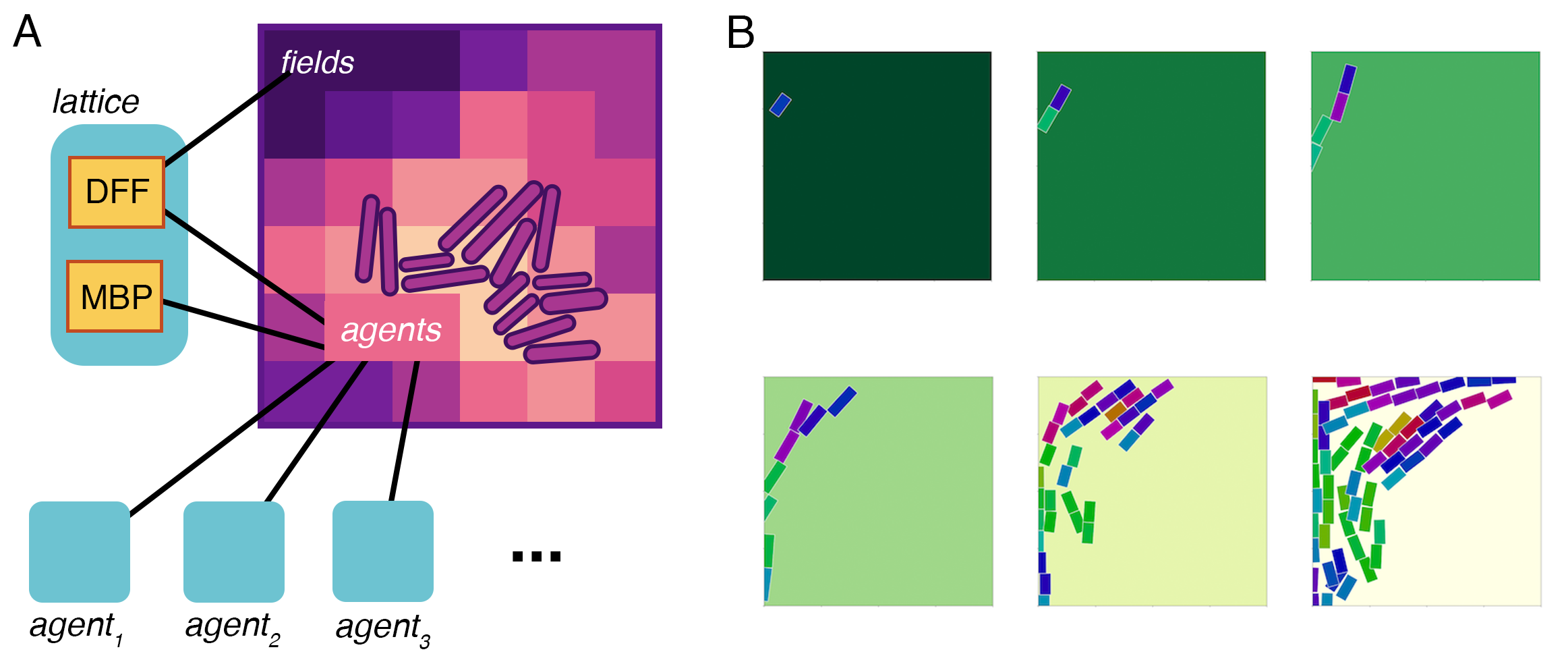
Combining Lattice, Diffusion, and Multi-Body Physics
Putting these three components together, we can simulate cells (agents) moved by multi-body physics (MBP) in a shared environment whose metabolite concentrations (fields) are diffused by a diffusion process (DFF):